Diffusion Models: A Comprehensive Survey of Methods and Applications

Diffusion models have emerged as a powerful new family of deep generative models with record-breaking performance in many applications, including image synthesis, video generation, and molecule design. In this survey, we provide an overview of the rapidly expanding body of work on diffusion models, categorizing the research into three key areas: efficient sampling, improved likelihood estimation, and handling data with special structures. We also discuss the potential for combining diffusion models with other generative models for enhanced results. We further review the wide-ranging applications of diffusion models in fields spanning from computer vision, natural language processing, temporal data modeling, to interdisciplinary applications in other scientific disciplines.

FOUNDATIONS OF DIFFUSION MODELS

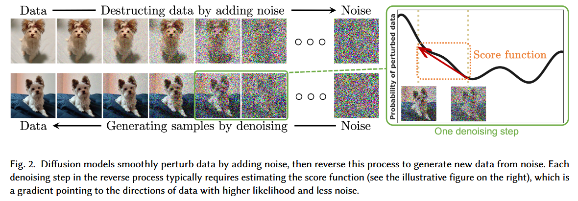
Diffusion models are a family of probabilistic generative models that progressively destruct data by injecting noise, then learn to reverse this process for sample generation. Current research on diffusion models is mostly based on three predominant formulations: denoising diffusion probabilistic models (DDPMs), score-based generative models (SGMs), and stochastic differential equations (Score SDEs).

Denoising Diffusion Probabilistic Models (DDPMs)

A denoising diffusion probabilistic model (DDPM) makes use of two Markov chains: a forward chain that perturbs data to noise, and a reverse chain that converts noise back to data.

Formally, given a data distribution $x_0 \sim q(x_0)$, the forward Markov process generates a sequence of random variables $x_1$, $x_2$ . . . $x_T$ with transition kernel $q(x_t \mid x_{t-1})$. The joint distribution of $x_1$, $x_2$ . . . $x_T$ conditioned on $x_0$, denoted as $q(x_1, . . . , x_T \mid x_0)$:

$$
q(x_1, . . . , x_T \mid x_0) = \prod_{i=1}^T q(x_t \mid x_{t-1}) \tag{1.1}
$$
One typical design for the transition kernel is Gaussian perturbation, and the most common choice for the transition kernel is
$$
q(x_t \mid x_{t−1}) = \mathcal{N} (x_t ; \sqrt{1 − \beta_t} x_{t−1} , \beta_t I) \tag{1.2}
$$
This Gaussian transition kernel allows us to marginalize the joint distribution in Eq. (1.1) to obtain the analytical form of $q(x_t \mid x_0)$ for all $t \in {0, 1, · · · ,T }$. Specifically, with $\alpha_t := 1 − βt$ and $\overline\alpha_t := \prod_{s=0}^t \alpha_s $, we have
$$
q(x_t \mid x_0) = \mathcal{N}(x_t; \sqrt{\overline\alpha_t} x_0, (1-\overline\alpha_t)I) \tag {1.3}
$$
Given $x_0$, we can easily obtain a sample of $x_t$ by sampling a Gaussian vector $\epsilon \sim \mathcal{N} (0, I)$ and applying the transformation
$$
x_t = \sqrt{\overline\alpha_t}x_0 + \sqrt{1-\overline\alpha_t}\epsilon \tag{1.4}
$$
The learnable transition kernel $p_{\theta} (x_{t−1} \mid x_t )$ takes the form of
$$
p_\theta(x_{t-1} \mid x_t) = \mathcal{N}(x_{t-1}; \mu_\theta(x_t, t), \Sigma_\theta(x_t, t)) \tag{1.5}
$$
where $\theta$ denotes model parameters, and the mean $ \mu_\theta(x_t , t)$ and variance $\Sigma_\theta(x_t , t)$ are parameterized by deep neural networks.

Key to the success of this sampling process is training the reverse Markov chain to match the actual time reversal of the forward Markov chain. This is achieved by minimizing the Kullback-Leibler (KL) divergence.

Ho et al. (2020) propose to reweight various terms in $L_{VLB}$ for better sample quality and noticed an important equivalence between the resulting loss function and the training objective for noise-conditional score networks (NCSNs), one type of score-based generative models, in Song and Ermon. The loss takes the form of
$$
\mathbb{E}_{t\sim\mathcal{U}[1, T], x_0\sim q(x_0), \epsilon\sim \mathcal{N}(0, I)}\left[\lambda(t)\Vert\epsilon - \epsilon_\theta(x_t, t)\Vert^2\right] \tag{1.6}
$$
where $\lambda(t)$ is a positive weighting function, $x_t$ is computed from $x_0$ and $\epsilon$ by Eq. (1.4), $\mathcal{U}[1, T]$ s a uniform distribution over the set ${1, 2, · · · ,T }$, and $\epsilon_\theta$ is a deep neural network with parameter $\theta$ that predicts the noise vector $\epsilon$ given $x_t$ and $t$.

Score-Based Generative Models (SGMs)

The key idea of score-based generative models (SGMs) is to perturb data with a sequence of intensifying Gaussian noise and jointly estimate the score functions for all noisy data distributions by training a deep neural network model conditioned on noise levels (called a noise-conditional score network, NCSN).

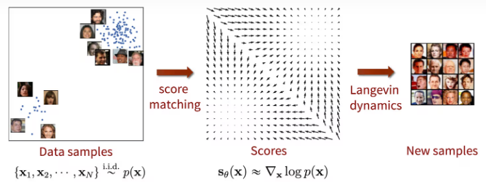
With similar notations in DDPMs, we let $q(x_0)$ be the data distribution, and $0 < \sigma_1 < \sigma_2 < · · · < \sigma_t < · · · < \sigma_T$ be a sequence of noise levels. A typical example of SGMs involves perturbing a data point $x_0$ to $x_t$ by the Gaussian noise distribution $q(x_t \mid x_0) = \mathcal{N} (x_t ; x_0, \sigma_t^2 I )$. This yields a sequence of noisy data densities $q(x_1), q(x_2), · · · , q(x_T )$.

With denoising score matching and similar notations in Eq. (1.6), the training objective is given by
$$
\mathbb{E}_{t\sim\mathcal{U}\text{〚}1, T \text{〛}, x_0\sim q(x_0), x_t\sim q(x_t\mid x_0)}\left[\lambda(t)\sigma_t^2\Vert \nabla_{x_t}\log {q(x_t)} - s_\theta(x_t, t) \Vert^2 \right] \tag{1.7}
$$
$$
= \mathbb{E}_{t\sim\mathcal{U}\text{〚}1, T \text{〛}, x_0\sim q(x_0), x_t\sim q(x_t\mid x_0)}\left[\lambda(t)\sigma_t^2\Vert \nabla_{x_t}\log {q(x_t|x_0)} - s_\theta(x_t, t) \Vert^2 \right] + const \tag{1.8}
$$
$$
= \mathbb{E}_{t\sim\mathcal{U}\text{〚}1, T \text{〛}, x_0\sim q(x_0), x_t\sim q(x_t\mid x_0)}\left[\lambda(t)\Vert -\frac{x_t - x_0}{\sigma_t} - \sigma_ts_\theta(x_t, t) \Vert^2 \right] + const \tag{1.9}
$$
$$
= \mathbb{E}_{t\sim\mathcal{U}\text{〚}1, T \text{〛}, x_0\sim q(x_0), \epsilon\sim \mathcal{N}(0, I)}\left[\lambda(t)\Vert \epsilon + \sigma_ts_\theta(x_t, t) \Vert^2 \right] + const \tag{1.10}
$$

Stochastic Differential Equations (Score SDEs)

DDPMs and SGMs can be further generalized to the case of infinite time steps or noise levels, where the perturbation and denoising processes are solutions to stochastic differential equations (SDEs). We call this formulation Score SDE, as it leverages SDEs for noise perturbation and sample generation, and the denoising process requires estimating score functions of noisy data distributions.

Score SDEs perturb data to noise with a diffusion process governed by the following stochastic differential equation (SDE):
$$
dx = f(x, t)dt + g(t)dw \tag{1.11}
$$
where $f (x, t) $and $g(t)$ are diffusion and drift functions of the SDE, and w is a standard Wiener process (a.k.a., Brownian motion). The forward processes in DDPMs and SGMs are both discretizations of this SDE. As demonstrated in Song et al. (2020), for DDPMs, the corresponding SDE is:
$$
dx = -\frac{1}{2}\beta(t)xdt + \sqrt{\beta(t)}dw \tag{1.12}
$$
where $\beta(\frac{t}{T}) = T\beta_t$ as $T$ goes to infinity; and for SGMs, the corresponding SDE is given by
$$
dx = \sqrt{\frac{d[\sigma(t)^2]}{dt}}dw \tag{1.13}
$$
where $\sigma(\frac{t}{T}) = \sigma_t$ as $T$ goes to infinity. Here we use $q_t (x)$ to denote the distribution of $x_t$ in the forward process.

Crucially, for any diffusion process in the form of Eq. (1.9), Anderson shows that it can be reversed by solving the following reverse-time SDE:
$$
dx = \left[f(x, t) - g(t)^2\nabla_x\log{q_t(x)}\right]dt+g(t)d\overline{w} \tag{1.14}
$$
where $\overline{w}$ is a standard Wiener process when time flows backwards, and $dt$ denotes an infinitesimal negative time step.

Moreover, Song et al. (2020) prove the existence of an ordinary differential equation (ODE), namely the probability flow ODE, whose trajectories have the same marginals as the reverse-time SDE. The probability flow ODE is given by:
$$
dx = \left[ f(x, t) - \frac{1}{2}g(t)^2\nabla_x\log{q_t(x)} \right]dt \tag{1.15}
$$
Both the reverse-time SDE and the probability flow ODE allow sampling from the same data distribution as their trajectories have the same marginals.

Like in SGMs, we parameterize a time-dependent score model $s_θ (x_t , t)$ to estimate the score function by generalizing the score matching objective to continuous time, leading to the following objective:
$$
\mathbb{E}_{t\sim\mathcal{U}[0, T], x_0\sim q(x_0), x_t\sim q(x_t\mid x_0)}\left[\lambda(t)\Vert s_\theta(x_t, t) - \nabla_{x_t}\log {q_{0t}(x_t\mid x_0)\Vert^2} \right] \tag{1.16}
$$
where $\mathcal{U}[0, T]$ denotes the uniform distribution over $[0,T ]$.

Subsequent research on diffusion models focuses on improving these classical approaches (DDPMs, SGMs, and Score SDEs) from three major directions: faster and more efficient sampling, more accurate likelihood and density estimation, and handling data with special structures (such as permutation invariance, manifold structures, and discrete data).